Sales Forecasting Predictions

This project takes 2.5 years of historical daily sales data (January 2013 – July 2015) from 1,115 Rossmann store locations and turns it into a working forecasting system. The pipeline covers the full lifecycle of a data science project: cleaning and joining raw data, engineering time-aware features, exploring trends through visualization, training and tuning an XGBoost regression model, rigorously evaluating its performance, and packaging the results into a Shiny app that lets a user pick any store and time window to compare actual vs. predicted sales. The motivation was to gain hands-on experience with two things at once: forecasting on time-series data and working with a gradient boosting model, using the well-known Kaggle Rossmann Store Sales competition as the testbed.

Retailers need accurate, forward-looking sales estimates at the individual store level to plan staffing, inventory, and promotions effectively. Sales are driven by a mix of factors that interact in non-obvious ways — day of week, promotions, competition, holidays, and recent sales momentum — which makes naive averages or simple trend lines unreliable. The goal was to build a model that predicts daily sales per store with meaningfully better accuracy than a baseline approach, while remaining interpretable and fast enough to serve interactively through a dashboard.

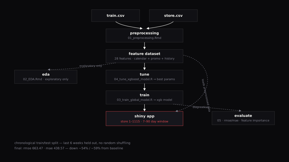
Joined the raw sales data with store metadata so every row represents a single store on a single day, imputing missing values in competition-related fields rather than dropping or zero-filling them (either choice would have biased the data or discarded a large share of rows), and adding missingness indicators for promo fields to preserve information about why a value was missing. Engineered calendar features (year, month, day, week, day-of-week, weekend/month-start/month-end flags), status flags (closed-day, promo active, competition active), and sales-history features (1/7/14-day lags, 7/14-day rolling means) to give the model a sense of recent momentum and local seasonality per store. Ran exploratory analysis with skimr and ggplot2/plotly to visualize daily sales trends, monthly seasonality, day-of-week patterns, and sales distributions across promo status, holidays, store type, and assortment type. Split the data chronologically, holding out the last six weeks as a test set — a random split would let the model 'see the future' through the lag and rolling features — then trained an XGBoost regressor on 28 features spanning calendar, promo, competition, and sales-history signals. Ran a grid search over eta, max depth, subsample, colsample_bytree, and rounds, evaluating each combination on the same time-based holdout and selecting the configuration with the lowest RMSE. Compared training vs. test RMSE/MAE to confirm the tuned model wasn't overfitting, then visualized residuals vs. predicted sales, actual vs. predicted sales, aggregate daily actual vs. predicted sales, a residual distribution histogram, and feature importance. Finally, built a Shiny dashboard so a non-technical user can select any store (1–1115) and a time window (7–90 days) and see actual vs. predicted sales plotted side by side, along with summary totals for the selected period.

Tuning and feature engineering together cut RMSE from 1433.87 to 663.47 (roughly 54%) and MAE from 1081.46 to 438.57 (roughly 59%) relative to the baseline. Training vs. test error was checked directly to confirm the improvement wasn't due to overfitting. The lag and rolling-average sales features, along with the closed-day and month-position indicators, were among the most influential in reducing error, since they gave the model direct signal about each store's recent momentum rather than relying solely on static, calendar-level information. The final model and dataset are served through a Shiny dashboard where a user can select any store and a 7–90 day window to visually compare actual and predicted sales and see aggregate totals for that period, turning the model from a static evaluation artifact into an explorable tool. Initial model performance was weak and was resolved through targeted feature engineering combined with systematic hyperparameter tuning; building the Shiny app itself was a new skill for this project, requiring learning reactive programming patterns to wire up the store/time-window inputs to live predictions and plots. Next steps: a reliable method for generating lag and rolling-average features for genuinely future dates, richer holiday-related time features, and incorporating geographic data per store.

outcome: Feature engineering and hyperparameter tuning together cut RMSE by ~54% (1433.87 → 663.47) and MAE by ~59% (1081.46 → 438.57) versus the baseline model.

• 

  Total sales, actual vs. predicted, aggregated by day — the same comparison the Shiny dashboard shows live.

• 

  Predicted vs. actual sales at the row level — tight clustering along the diagonal across 20,000+ test predictions.

• 

  Top 20 feature importances — Open, 7-day rolling mean, and 14-day lag dominate the model's decisions.

• XGBoost
• R
• Shiny
• ggplot2
• tidyverse